Spiketimes Numpy Tutorial
The easiest way to get started with spiketimes is by working with numpy arrays. In this framework, a spiketrain is represented as a numpy array of spike times in seconds.
Generating Spiketrains
Spiketrains can be generated by simulation, or creation of surrogates of existing spiketrains or by loading in data files.
Simulating Spiketrains
The spiketimes.simulate module contains functions for simulating spiketrains.
Lets simulate an irregular-spiking spiketrain with a constant firing rate. For this, we’ll use the spiketimes.simulate.homogeneous_poisson_process() function.
>>> from spiketimes.simulate import homogeneous_poisson_process
>>>
>>> st = homogeneous_poisson_process(rate=4, t_start=8, t_stop=10)
>>> st
array([8.05172817, 8.15086753, 8.22174441, 8.44837953, 8.66746485,
   8.7746017 , 8.94102246, 8.97722358, 9.2492881 , 9.52008361,
   9.5500119 , 9.7534826 , 9.83049717, 9.88975479])
We can also simulate spiketrains that change their firing rate over time. For example:
>>> from spiketimes.simulate import imhomogeneous_poisson_process
>>>
>>>
>>> imhomogeneous_poisson_process(time_rate=[(5, 0.5), (2, 5)], t_start=1)
array([1.3895191 , 2.75733416, 3.79203384, 6.0275662 , 6.26492861,
   6.27737558, 6.57495924, 6.6764454 , 6.70029706, 6.76780677,
   6.96170539, 7.54483481, 7.56002437, 7.69575184, 7.74121035,
   7.92529903])
Generating Spiketrain Surrogates
The spiketimes.surrogates module contains functions for generating spiketrain surrogates. Surrogate spiketrains are randomly generated spiketrains which share some properties with a parent spiketrain but are otherwise different. They are often used for generating bootstrap replicates.
One of the most common types of spiketrain surrogates are shuffled inter-spike-interval (isi) surrogates. These spiketrains have identical isi distrobutions to their parent, but with shuffled order. They can be generated in spiketimes using the spiketimes.surrogates.shuffled_isi_spiketrain(): function.
>>> from spiketimes.simulate import homogeneous_poisson_process
>>> from spiketimes.surrogates import shuffled_isi_spiketrain
>>>
>>> original_spiketrain = homogeneous_poisson_process(rate=0.5, t_stop=30)
>>> shuffled = shuffled_isi_spiketrain(original_spiketrain)
Jitter spiketrains are another common type of spiketrain surrogate. They share a similar pattern of time-varying firing rate as their parent, but with offset spiketimes. They can be generated in spiketimes using the spiketimes.surrogates.jitter_spiketrain(): function.
>>> from spiketimes.surrogates import jitter_spiketrain
>>>
>>> jittered = jitter_spiketrain(original_spiketrain, jitter_window_size=0.5)
Aligning and Binning Data
One of the most common tasks in analysis of neuroscience experimental data is aligning data to events. The spiketimes.alignment and spiketimes.binning modules contain functions to align and bin data.
Data can be easily aligned to events using the spiketimes.alignment.align_around() function. This function is highly customisable. Check out all of its options in the API Reference. See below for an example:
>>> from spiketimes.simulate import homogeneous_poisson_process
>>> from spiketimes.alignment import align_around
>>> import numpy as np
>>>
>>>
>>> events = np.arange(start=2, stop=14, step=4)
>>> print(f"Events: \t{events}")
Events:     [ 2  6 10]
>>> st = homogeneous_poisson_process(rate=1, t_stop=14, t_start=1)
>>> print(f"Spiketimes: \t{st}")
Spiketimes:         [ 1.80323015  1.84967261  2.03991789  2.07067261  2.28136596  3.08029239
3.30143406  3.63229053  4.08733938  4.17661091  4.86958822  5.51102716
6.60802296  7.8849845   8.12873198 10.48377187 10.93672175 11.04330173
11.30156375 11.34996232 11.59105221 11.90801207]
>>> aligned_spiketimes = align_around(st, events, t_before=1, max_latency=5)
>>> print(f"Aligned Spiketimes: \t{aligned_spiketimes}")
Aligned Spiketimes:         [-0.19676985 -0.15032739  0.03991789  0.07067261  0.28136596  1.08029239
1.30143406  1.63229053  2.08733938  2.17661091  2.86958822 -0.48897284
0.60802296  1.8849845   2.12873198  0.48377187  0.93672175  1.04330173
1.30156375  1.34996232  1.59105221  1.90801207]
Spiketrains can be split into lists of spiketrains by trial using the spiketimes.alignment.split_by_trial() function:
>>> from spiketimes.alignment import split_by_trial
>>>
>>> trial_starts = np.array([5, 10])
>>> st_list = split_by_trial(spiketrain=st, trial_starts=trial_starts)
To get spike counts at regular time bins, use the spiketimes.alignment.binned_spiketrain() function.
>>> from spiketimes.alignment import binned_spiketrain
>>> from spiketimes.simulate import homogeneous_poisson_process
>>>
>>> st = homogeneous_poisson_process(rate=4, t_start=0, t_stop=4)  # spiketrain with a constant 4Hz Firing rate
>>> fs = 1  # sampling rate of binning (1 / bin width)
>>> bin_edges, spike_counts = binned_spiketrain(st, fs=fs, t_start=0)
>>> print(f"Edges: \t{bin_edges}")  # bin_edges contain the right edges of the bins
Edges:      [1. 2. 3. 4.]
>>> print(f"Spike Counts: \t {spike_counts}")  # spike_counts contains the number of spikes falling in that bin
Spike Counts:        [6 1 8 2]
Or to get spike counts at arbitrary time bins, use the spiketimes.alignment.binned_spiketrain_bins_provided() function:
>>> from spiketimes.alignment import binned_spiketrain_bins_provided
>>> import numpy as np
>>>
>>> bins = np.arange(start=0, stop=4, step=0.02)
>>> binned_st = binned_spiketrain_bins_provided(spiketrain=st, bins=bins)
To get spike counts in a time window following events, use the spiketimes.alignment.spike_count_around_event() function:
>>> from spiketimes.alignment import spike_count_around_event
>>>
>>> events = np.array([1.1, 2.4])  # event times in seconds
>>> spike_counts = spike_count_around_event(spiketrain=st, events=events, binsize=0.3)
Statistics
The spiketimes.statistics provides a variety of functions for calculating spiketrain descriptive statistics.
To calculate the mean firing rate of a neuron, use the spiketimes.statistics.mean_firing_rate() function:
>>> from spiketimes.statistics import mean_firing_rate
>>> from spiketimes.simulate import homogeneous_poisson_process
>>>
>>> st = homogeneous_poisson_process(rate=10, t_start=0, t_stop=120)  # neuron firing at 10Hz for 2 minutes
>>> mean_firing_rate(st)
10.13083858467599
To get a time-varying estimate of a neurons firing rate, use the spiketimes.statistics.ifr() function:
>>> from spiketimes.statistics import ifr
>>>
>>> fs = 1  # sampling rate at which to estimate firing rate
>>> time_bins, firing_rate = ifr(st, fs=fs, as_df=False)
To get the inter-spike-intervals of a spiketrian, use the spiketimes.statistics.inter_spike_intervals() function.
>>> from spiketimes.statistics import inter_spike_intervals
>>> from spiketimes.simulate import homogeneous_poisson_process
>>>
>>> st = homogeneous_poisson_process(rate=30, t_stop=60)
>>> isi = inter_spike_intervals(st)
To calculate the coeficient of variation of inter-spike-intervals (a metric of spike regularity), use spiketimes.statistics.cv_isi().
>>> from spiketimes.statistics import cv_isi
>>>
>>> cv_isi(st)
0.988
Correlating Spiketrains
The spiketimes.correlate module contains functions for correlating spiketrains.
To correlate spike counts in pairs of neurons, use spiketimes.correlate.spike_count_correlation():
>>> from spiketimes.correlate import spike_count_correlation
>>> from spiketimes.simulate import imhomogeneous_poisson_process
>>>
>>> # generate two spiketrains which shift their firing rates simultaneously
>>> time_rate = [
>>>     (120, 3),
>>>     (60, 5),
>>>     (120, 8),
>>>     (60, 2),
>>>     (120, 10)
>>> ]
>>> st1 = imhomogeneous_poisson_process(time_rate=time_rate)
>>> st2 = imhomogeneous_poisson_process(time_rate=time_rate)
>>>
>>> fs = 10  # sampling rate at which to use for correlation (1/binsize)
>>> spike_count_correlation(st1, st2, binsize=0.1)
0.1167
To test the significance of a correlation:
>>> from spiketimes.correlate import spike_count_correlation_test
>>>
>>> r, p = spike_count_correlation_test(st1, st2, binsize=binsize, n_boot=5000)
>>> (r, p)
(0.1167, 0.0272)
To calculate’s a spiketrain’s autocorrelation histogram, use the spiketimes.correlate.auto_corr() function:
>>> from spiketimes.correlate import auto_corr
>>>
>>> bins, values = auto_corr(st1, binsize=0.01, num_lags=50)
To calculate the crosscorelation histogram between two spiketrains, use the spiketimes.correlate.cross_corr() function:
>>> from spiketimes.correlate import cross_corr
>>>
>>> bins, values = cross_corr(st1, st2, binsize=0.01, num_lags=50)
Plots
The spiketimes.plots module contains functions for plotting spiketrains.
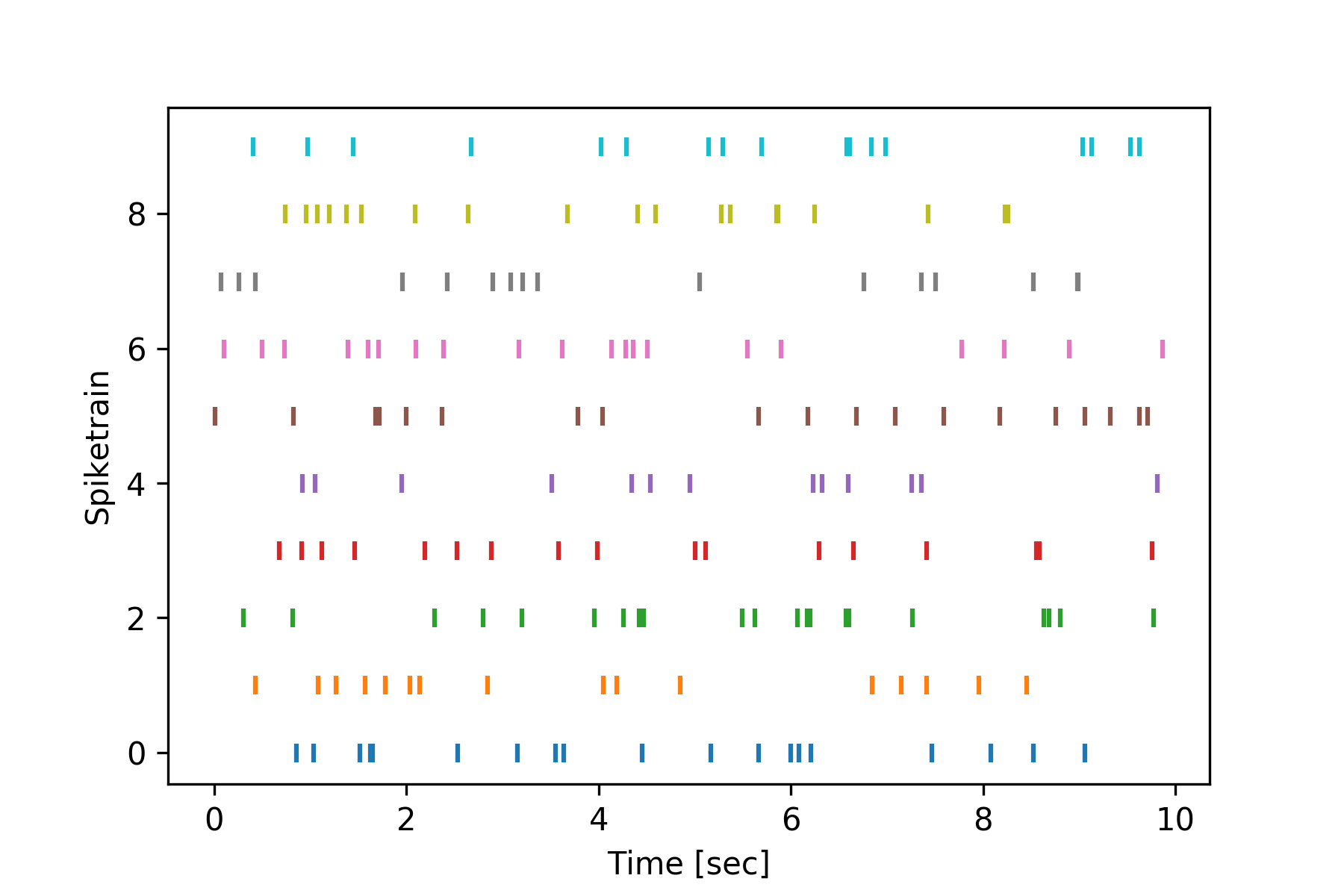
To plot a raster containing multiple spiketrains, use the spiketimes.plots.raster() function:
>>> from spiketimes.plots import raster
>>>
>>>
>>> # create list of spiketrains firing at 2Hz for 10 seconds
>>> spiketrain_list = [homogeneous_poisson_process(rate=2, t_start=0, t_stop=10) for _ in range(10)]
>>>
>>> f, ax = plt.subplots()
>>> ax = raster(spiketrain_list, ax=ax)  # create the plot
>>> plt.show()
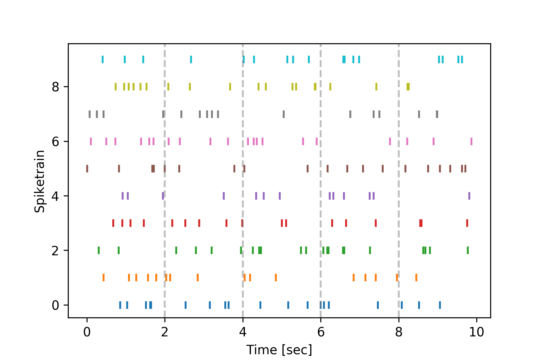
You can indicate event times by adding vertical lines to plots using the spiketimes.plots.add_event_vlines() function:
>>> from spiketimes.plots import add_event_vlines
>>> import numpy as np
>>>
>>>
>>> events = np.array([2, 4, 6, 8])
>>>
>>> f, ax = plt.subplots()
>>> ax = raster(spiketrain_list, ax=ax)  # create the initial plot
>>> # add vertical lines indicating event timings
>>> ax = add_event_vlines(ax=ax, events=events, vline_kwargs={"alpha": 0.5})
>>> plt.show()
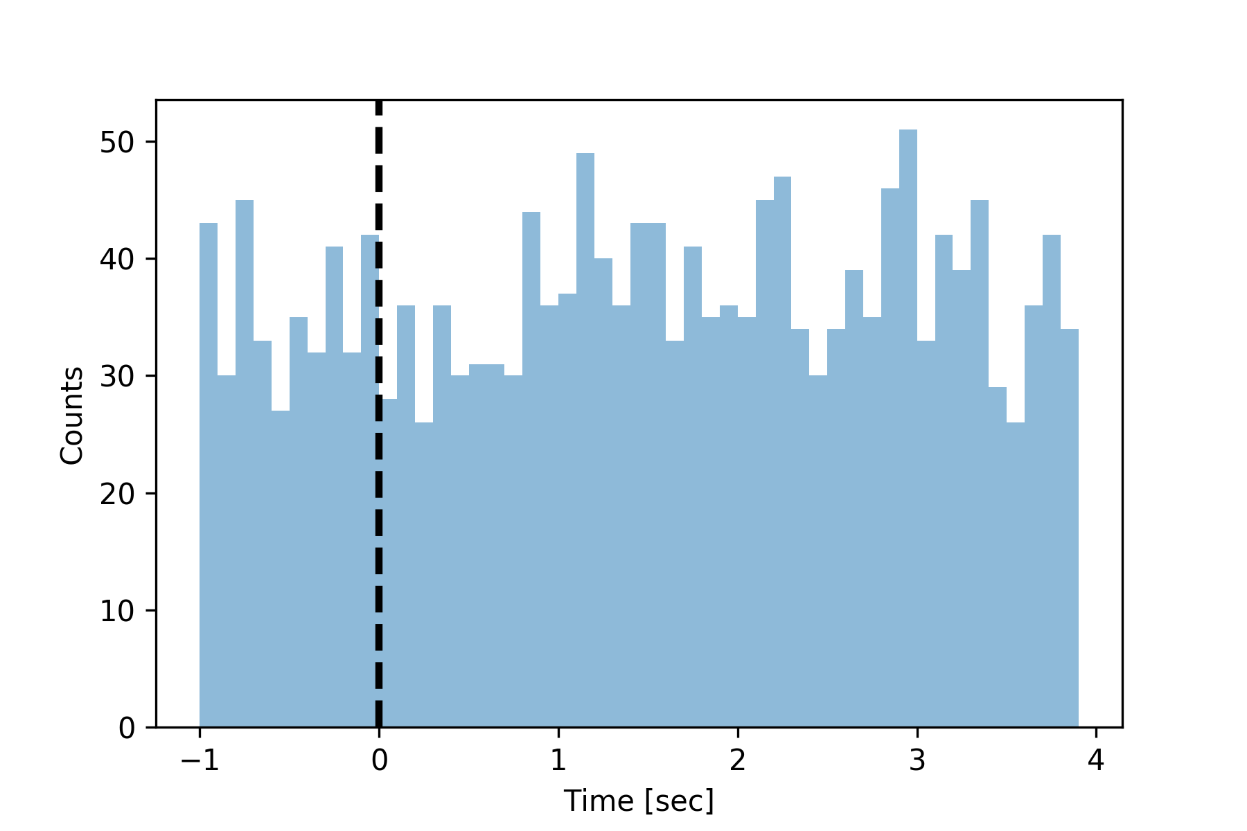
Construct peri-stimulus time histograms using the spiketimes.plots.psth() function.
>>> from spiketimes.plots import psth, add_event_vlines
>>>
>>> # generate random neuron
>>> st = homogeneous_poisson_process(rate=10, t_stop=1000)
>>>
>>> # generate some events
>>> events = np.arange(0, 180, 5)
>>>
>>> # plot the psth
>>> ax = psth(st, events, binwidth=0.1, t_before=1, max_latency=4)